This article is also available on Medium, you can click here to read it there.
Marketing has evolved far beyond simple click-through rates and conversion tracking. Today’s performance marketers need to understand concepts like customer lifetime value (LTV), return on ad spend (ROAS), customer segmentation and sophisticated attribution modeling. I’ve found (finally!) that organisations are holding marketers and agencies accountable for marketing performance – and NO, this wasn’t always the case – I’ve lived it and dealing with a smug ad agency that would not be held accountable for poor performance because their address was on Madison Avenue was the bane of my existance for some time.
In this series, I will walk you through the essential performance marketing concepts and show you how to calculate performance metrics. The concepts I’m going to cover over the next 11 or so articles are the following (there’s 11 concepts, so probably 11 articles):
- CPA (Cost Per Acquisition) – Channel efficiency analysis – one of the most important performance marketing metrics, representing the total cost to acquire one customer or conversion action.
- ROAS (Return on Ad Spend) – Campaign profitability measurement – a revenue efficiency metric that measures how much revenue is generated for every dollar spent on advertising.
- LTV (Customer Lifetime Value) – Predictive customer valuation – measures the total net profit a customer generates over their entire relationship with your business. It’s the foundation for determining how much you can afford to spend acquiring customers.
- Cohort Analysis – Customer behavior tracking over time – a method of grouping customers by shared characteristics (typically acquisition date) and tracking their behavior over time to understand patterns in retention, revenue, and lifetime value.
- Contribution Margin – True profitability assessment – the profit remaining after subtracting variable costs from revenue. It represents the amount available to cover fixed costs and generate profit, and critically for performance marketing, it determines how much you can afford to spend on customer acquisition.
- Customer Segmentation – RFM and behavioral clustering – the practice of dividing your customer base into distinct groups that share similar characteristics, behaviors, or value profiles—enabling targeted strategies that improve acquisition efficiency, retention, and lifetime value.
- Churn Prediction – Machine learning models for retention – uses historical customer behavior data to identify which customers are most likely to stop doing business with you, enabling proactive retention interventions before they leave.
- Personalized Offer Scoring – Targeted campaign optimization – predicts which specific offer (discount level, product, message, timing, channel) to present to each individual customer to maximize business outcomes while minimizing unnecessary cost—essentially applying incrementality principles at the individual customer level.
- Attribution Modeling – Multi-touch attribution including Markov chains – assigns credit for conversions across the multiple marketing touchpoints a customer encounters along their journey to purchase. It attempts to answer: “Which marketing activities actually drove this conversion?”
- Cohort-Based LTV – Advanced lifetime value forecasting – measures the actual lifetime value of customers grouped by a shared characteristic (typically acquisition date or channel), tracking their real revenue and behavior over time rather than relying on aggregate or modeled estimates.
- Order Economics – Transaction-level profitability analysis – the complete financial breakdown of an individual transaction—all revenue, costs, and resulting profit from a single order.
I decided to break this up so it’s not one giant article, but a series of smaller, more digestable articles (also so that I can feel that I’m actually accomplishing something since I haven’t published anything for about 10 months – I’ve got parts of about 10 different articles I have yet to finish).
Setting Up Our Sample Dataset
But first, we need some marketing data. There are many souces of free datasets, but I sometimes feel it can be best to create your own. So, the first step is to create a realistic e-commerce dataset that mirrors what you’d find in most marketing databases. We’ll build several interconnected tables that capture the customer journey from first touch to repeat purchases.
SQL Schema and Sample Data
I’m going to write out some SQL that you can use to create a few tables, create relationships between them, and load some data. If you’ve never used SQL, welcome! This will be fun and as a performance marketer, SQL will be one of your best friends. Of course, I could have just used Python and created the tables that way, but that’s not where you’ll find most marketing data. They’re usually in BigQuery or Snowflake and they mostly just understand SQL.
This will work in any database system and you can just copy & paste the following into an IDE like DBeaver (which is FREE, or more accurately, open source and my favourite IDE and I’ve tried practicaly all of them) or anywhere that you can run SQL – some bold individulas just use a command line. I find that to be fairly unproductive overall (use an IDE). You should end up with four related tables and 5-10 rows of data, depending on the table.
-- Create customers table
CREATE TABLE customers (
    customer_id INT PRIMARY KEY,
    first_purchase_date DATE,
    acquisition_channel VARCHAR(50),
    customer_segment VARCHAR(50),
    registration_date DATE
);

-- Create orders table
CREATE TABLE orders (
    order_id INT PRIMARY KEY,
    customer_id INT,
    order_date DATE,
    order_value DECIMAL(10,2),
    product_cost DECIMAL(10,2),
    shipping_cost DECIMAL(10,2),
    FOREIGN KEY (customer_id) REFERENCES customers(customer_id)
);

-- Create marketing_spend table
CREATE TABLE marketing_spend (
    date DATE,
    channel VARCHAR(50),
    spend DECIMAL(10,2),
    impressions INT,
    clicks INT
);

-- Create attribution_touchpoints table
CREATE TABLE attribution_touchpoints (
    touchpoint_id INT PRIMARY KEY,
    customer_id INT,
    channel VARCHAR(50),
    touchpoint_date DATE,
    conversion_value DECIMAL(10,2),
    position_in_journey INT,
    FOREIGN KEY (customer_id) REFERENCES customers(customer_id)
);

-- Insert sample customers data
INSERT INTO customers VALUES
(1, '2023-01-15', 'google_ads', 'high_value', '2023-01-15'),
(2, '2023-01-16', 'facebook_ads', 'medium_value', '2023-01-16'),
(3, '2023-01-17', 'organic_search', 'high_value', '2023-01-17'),
(4, '2023-01-18', 'email_marketing', 'low_value', '2023-01-18'),
(5, '2023-01-19', 'google_ads', 'medium_value', '2023-01-19'),
(6, '2023-01-20', 'facebook_ads', 'high_value', '2023-01-20'),
(7, '2023-01-21', 'organic_search', 'medium_value', '2023-01-21'),
(8, '2023-01-22', 'email_marketing', 'low_value', '2023-01-22'),
(9, '2023-01-23', 'google_ads', 'high_value', '2023-01-23'),
(10, '2023-01-24', 'facebook_ads', 'medium_value', '2023-01-24');

-- Insert sample orders data
INSERT INTO orders VALUES
(1, 1, '2023-01-15', 150.00, 75.00, 10.00),
(2, 1, '2023-02-15', 200.00, 100.00, 10.00),
(3, 2, '2023-01-16', 80.00, 40.00, 8.00),
(4, 3, '2023-01-17', 300.00, 150.00, 15.00),
(5, 3, '2023-03-17', 250.00, 125.00, 12.00),
(6, 4, '2023-01-18', 45.00, 22.50, 5.00),
(7, 5, '2023-01-19', 120.00, 60.00, 10.00),
(8, 6, '2023-01-20', 400.00, 200.00, 20.00),
(9, 7, '2023-01-21', 180.00, 90.00, 12.00),
(10, 8, '2023-01-22', 60.00, 30.00, 8.00);

-- Insert marketing spend data
INSERT INTO marketing_spend VALUES
('2023-01-15', 'google_ads', 500.00, 10000, 200),
('2023-01-16', 'facebook_ads', 300.00, 8000, 150),
('2023-01-17', 'organic_search', 0.00, 5000, 250),
('2023-01-18', 'email_marketing', 100.00, 2000, 100),
('2023-01-19', 'google_ads', 600.00, 12000, 240),
('2023-01-20', 'facebook_ads', 400.00, 9000, 180);

-- Insert attribution touchpoints
INSERT INTO attribution_touchpoints VALUES
(1, 1, 'google_ads', '2023-01-14', 150.00, 1),
(2, 1, 'facebook_ads', '2023-01-15', 150.00, 2),
(3, 2, 'facebook_ads', '2023-01-16', 80.00, 1),
(4, 3, 'organic_search', '2023-01-16', 300.00, 1),
(5, 3, 'email_marketing', '2023-01-17', 300.00, 2);Code language: JavaScript (javascript)
There should be four related tables with data in each (unless something went horribly wrong): customers, orders, marketing_spend, and attribution_touchpoints. I created this in a local PostgresSQL database, which is a free RDBMS that you can install directly on your laptop. One of the alternative ways of working with SQL data is by using DuckDB, which runs directly embedded in a Python process without requiring a separate database server.
Ok, now that we have our marketing data ready, it’s time to dive into our first concept and the one we’ll concentrate on in this article – CPA or Cost Per Acquisition.
Cost Per Acquisition (CPA) Analysis
You spent a bunch of money on display ads, search ads and pre-roll videos. You worked with influencers and ran affiliate marketing campaigns. Now Finance is knocking on your door, asking if all that money did anything for the organisation. Did you tag all the ads? How did you track influencer & affiliate promotions? Oh, you didn’t? Oh, you tracked the easy stuff, but not the other, more challenging marketing activities, so you’re just going to ask Finance to trust you 🥴
There’s your first challenge – before we get to MMM or MTA, you need to have a measurement strategy. That’s why I’m an analytics first kinda marketeer – without the right data, you won’t get the rignt information, then you won’t make the right decisions, which will not lead to the right outcomes.
Once you are able to measure everything – all the ads, promotional activities, & sales – you need to tie them together and distribute credit for sales. That’s your marketing measurement strategy. Luckily, for CPA, you don’t need to do all that. You just need to know how much you spent and how many sales you made in a given period: CPA = Total Marketing Spend / Number of New Customers Acquired
CPA by Channel?
But hold on! You (and Finance) want to know the CPA by each channel so you know where to put more of your money. So, we’ll need to take this a step further. But what does that mean? Seems simple enough – just segment by channel and calculate CPA. But what if multiple channels ultimately drove a given sale? Shouldn’t they each have a slice of that sale. But how much? If they were the last channel that drove the sale, should they get most, all, some percentage of that sale? You can see where this gets complicated, quickly.
Luckily for us, I’ve sorted that out in our simple, fake data. IRL, this is all part of your measurement stratgy (I’ll probably do an article on that topic one day). If you are using a data lake or a platform that already calculates multi-channel attribution, this may have already been figured out for you. Then we can just add up the marketing spend and divide by the number of sales by channel (attribution touchpoints).
Actually Calculating CPA
We’re going to calculate CPA by channel. Then create a graph with the data. And finally, we’re going to calculate an upper and lower confidence interval (CI) and create a table with the channel, CPA, Upper Confidence Interval (UCI), Lower Confidence Interval (LCI) and Total Spend.
There are so many ways to calculate CPA once you have the data. We could just use Excel – pull the data out of the database (or ask someone in IT to do it), then work with it in Excel until we get what we need. The downside is that it’s all manual and there is minimal scalability. We’ll also need to do it over again for any new data. You can actually do this in BigQuery, but it’ll be locked in BigQuery and hard to share easily. We could also do it in R, and that’s a great idea. However, Python is taking over the world, so we’re going to do it in Python. It’s scalable, portable, and easily shared with others. Also, if you add more analysis, you can easily rerun the code as many times as you like.
Setting Up to Code CPA
We’re going to get a few things that we need for this calculation. Once you’ve downloaded Ptyhon and got it working (if you haven’t already), we’re going to import a few packages. These are some extra code to help us calculate the CPA. Next to each package I have entered a comment to tell you what each does. If you’re having trouble installing these packages or getting Python set up, I would recommend using Claude AI – it can really help you set everything up.
import pandas as pd # For data tables.
import numpy as np # For data arrays and typed data.
import matplotlib.pyplot as plt # To plot data.
import seaborn as sns # For stats visualisation.
from datetime import datetime, timedelta # For datetime data.
import psycopg2 #  PostgreSQL database adapter for Python.Code language: PHP (php)
Once the packages are imported, we’re going to make a connection to the database (wherever you have the data stored). Mine is in a local PostgreSQL database, so I can share my user name and password (usually this is a very big no no). I’m going to assign the connection to a variable conn:
# Create connection to db using psycopg2.
# SQLAlchemy is another, preferred way to connect, FYI.
conn = psycopg2.connect(
    host="localhost",
    database="postgres",
    user="postgres",
    password="Data123",
    port="5432"
)Code language: PHP (php)
Now I can load the marketing data into my Python IDE space. I’m going to do that by once again using SQL and selecting each dataset by writing a query and passing that to PostgreSQL. I can do that by using the pandas read_sql_query function and passing the query as a string and the connection conn we made above. That will create four pandas dataframes. Isn’t that cool!
# Open cursor and test connection.
cursor = conn.cursor()
cursor.execute("SET search_path TO 'marketing_guide'")

# Get the data from the tables and assign a dataframe variable to each.
customers = pd.read_sql_query("SELECT * FROM marketing_guide.customers", conn)
marketing_spend = pd.read_sql_query("SELECT * FROM marketing_guide.marketing_spend", conn)
orders = pd.read_sql_query("SELECT * FROM marketing_guide.orders", conn)
attribution_touchpoints = pd.read_sql_query("SELECT * FROM marketing_guide.attribution_touchpoints", conn)Code language: PHP (php)
Once we’ve got our data, we need to close our connection. For reference, if you don’t close your connections, you might get a visit from someone in IT, maybe a DBA, asking about all the connections you’ve opened. 😮
# Close cursor & connection.
cursor.close()
conn.close()Code language: CSS (css)
Creating CPA Function
Whew! Now we’re ready to roll up our sleeves and do some calculating. One way we can start is to create a reusable bit of code that can be called later, instead of writing it out each time. This is best when you do find yourself calculating the same thing over and over.
We’re going to create a function and name it calculate_cpa. We are going to have two variables that we can pass into this function – the marketing_spend dataframe and the customers dataframe. Those will become the variables spend_data and customer_data so as not to confuse them with the dataframes outside of the function. Also, we’re going to make some changes then return some data.
Okay, so to create a function, we use def then the fuction name, parenthesis, and in the parenthesis, the variables we’re passing into the function. Variables can be almost anything and you don’t have to declare what it is. This is something called duck typing – “If it walks like a duck and quacks like a duck, then it’s a duck”.
# Calculate CPA by channel
def calculate_cpa(spend_data, customer_data):
    # Group spending by channel
    spend_by_channel = spend_data.groupby('channel')['spend'].sum().reset_index()

    # Count customers by acquisition channel
    customers_by_channel = customer_data['acquisition_channel'].value_counts().reset_index()
    customers_by_channel.columns = ['channel', 'customer_count']

    # Merge and calculate CPA
    cpa_data = spend_by_channel.merge(customers_by_channel, on='channel', how='left')
    cpa_data['cpa'] = cpa_data['spend'] / cpa_data['customer_count']
    #cpa_data['efficiency_score'] = 1 / cpa_data['cpa']

    return cpa_dataCode language: PHP (php)
So we’re simply summing up the spend by channel, counting customers by channel, combining those two, then calculating the CPA. Having this as a function allows us to call it with any data in the marketing_spend and customers tables.
Let’s call it and print the results:
cpa_analysis = calculate_cpa(marketing_spend, customers)
print("CPA Analysis by Channel:")
print(cpa_analysis)Code language: PHP (php)
CPA Analysis by Channel:
channel spend customer_count cpa
0 email_marketing 100.0 2 50.000000
1 facebook_ads 700.0 3 233.333333
2 google_ads 1100.0 3 366.666667
3 organic_search 0.0 2 0.000000Code language: CSS (css)Building a CPA Chart
So that are the results in a simple output. Next, we want to create a bar chart with the CPA on the Y axis and the marketing channel on the X axis. We can do that by using the matplotlib.pyplot that we loaded up earlier and named plt.
There’s a bunch of functions and options with pyplot, like there is with any plotting packages. Here we’re going to just give it the basics – the size of the plot, the type of plot (you may have noticed, we’re using seaborn here since it requires less code than pure pyplot), with the X & Y axis, the title, and the lables for the X and Y axises. We’re also going to rotate the X axis 45 degrees since the names are a little long. We’re also going to make sure there’s no overlapping elements by adding tight_layout(). Finally, we add show() to view the plot.
# Sort by CPA ascending (best to worst)
cpa_analysis_sorted = cpa_analysis.sort_values('cpa', ascending=True)

# Visualize CPA
plt.figure(figsize=(12, 6))
sns.barplot(data=cpa_analysis_sorted, x='channel', y='cpa', palette='viridis')
plt.title('Cost Per Acquisition by Marketing Channel')
plt.xlabel('Marketing Channel')
plt.ylabel('CPA ($)')
plt.xticks(rotation=45)
plt.tight_layout()
plt.show()Code language: PHP (php)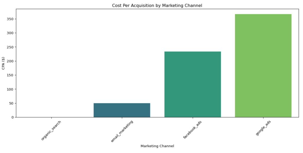
Adding Confidence Intervals to Our CPA Chart
We can get more sophisticated by adding confidence intervals to our data. The reason to do this is to look really smart 😬, and to show the variance in the data (instead of just the averages). This will give you an idea of how variable the CPA is. For example, you may have two marketing channels, both have a CPA of $200. However, one has wild swings from one period to anonther, while the other does not. The additional information of the confidence intervals can help you, first, understand channel behavior, and second, make more informed choices between the two channels.
# Advanced CPA analysis with confidence intervals
def cpa_with_confidence(spend_data, customer_data, confidence=0.95):
    """Resamples both spend and customers"""

    results = []

    for channel in spend_data['channel'].unique():
        # Get all spend observations (not just sum)
        channel_spend_values = spend_data[spend_data['channel'] == channel]['spend'].values
        channel_customers = len(customer_data[customer_data['acquisition_channel'] == channel])

        if channel_customers > 0:
            cpa = channel_spend_values.sum() / channel_customers

            # Bootstrap with resampling
            n_bootstrap = 1000
            bootstrap_cpas = []

            for _ in range(n_bootstrap):
                # Resample spend observations with replacement
                sample_spend = np.random.choice(channel_spend_values,
                                                size=len(channel_spend_values),
                                                replace=True).sum()

                # Resample customer count from Poisson
                sample_customers = np.random.poisson(channel_customers)

                if sample_customers > 0:
                    bootstrap_cpa = sample_spend / sample_customers
                    bootstrap_cpas.append(bootstrap_cpa)

            ci_lower = np.percentile(bootstrap_cpas, (1 - confidence) / 2 * 100)
            ci_upper = np.percentile(bootstrap_cpas, (1 + confidence) / 2 * 100)

            results.append({
                'channel': channel,
                'cpa': cpa,
                'ci_lower': ci_lower,
                'ci_upper': ci_upper,
                'ci_width': ci_upper - ci_lower,  # Useful metric
                'total_spend': channel_spend_values.sum(),
                'total_customers': channel_customers
            })

    return pd.DataFrame(results)Code language: PHP (php)
cpa_confidence = cpa_with_confidence(marketing_spend, customers)
print("\nCPA with 95% Confidence Intervals:")
print(cpa_confidence)Code language: PHP (php)
CPA with 95% Confidence Intervals:
           channel         cpa    ci_lower  ci_upper     ci_width  \
0       google_ads  366.666667  157.142857    1200.0  1042.857143
1     facebook_ads  233.333333   97.777778     800.0   702.222222
2   organic_search    0.000000    0.000000       0.0     0.000000
3  email_marketing   50.000000   20.000000     100.0    80.000000

   total_spend  total_customers
0       1100.0                3
1        700.0                3
2          0.0                2
3        100.0                2  Code language: CSS (css)
A lower CPA indicates more efficient customer acquisition, but it should always be evaluated against customer lifetime value to ensure profitability.
# Sort by CPA
cpa_confidence_sorted = cpa_confidence.sort_values('cpa', ascending=True)

plt.figure(figsize=(12, 6))

# Create the barplot
ax = sns.barplot(
    data=cpa_confidence_sorted,
    x='channel',
    y='cpa',
    palette='viridis'
)

# Add error bars for confidence intervals
x_coords = range(len(cpa_confidence_sorted))
plt.errorbar(
    x=x_coords,
    y=cpa_confidence_sorted['cpa'],
    yerr=[
        cpa_confidence_sorted['cpa'] - cpa_confidence_sorted['ci_lower'],  # Lower error
        cpa_confidence_sorted['ci_upper'] - cpa_confidence_sorted['cpa']   # Upper error
    ],
    fmt='none',          # No line connecting points
    ecolor='black',      # Error bar color
    capsize=5,           # Width of error bar caps
    capthick=2,          # Thickness of error bar caps
    elinewidth=2         # Thickness of error bar lines
)

plt.title('Cost Per Acquisition by Marketing Channel (with 95% CI)')
plt.xlabel('Marketing Channel')
plt.ylabel('CPA ($)')
plt.xticks(rotation=45)
plt.tight_layout()
plt.show()Code language: PHP (php)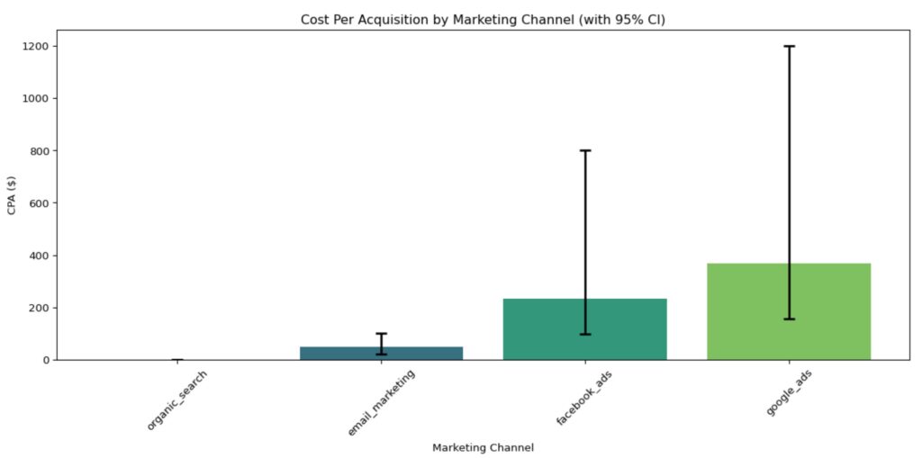
Conclusion
So that’s it – that’s CPA and how to calculate it (in Python). We created a dataset, calculated CPA by channel in a way that it can be rerun easily with new data, then we added a confidence interval by bootstraping our tiny dataset and calculating the upper and lower bound of the interval by channel. We then added that into our graph.
I hope you enjoyed this article and are feeling 👍 about it. My next article in this series will be about ROAS (Return on Ad Spend). Stay tuned!
About Us
We are Digital & Performance Marketing professionals. We help clients align marketing data, strategy & growth so that every decision, channel, and investment work together. If your data is disconnected, your strategy seems to be drifting, and your growth has been stalling, contact us today – we can help!