This article is also available on Medium.
This is a 2nd in an 11 part series of articles on marketing performance. In Pt. 1, we created a dataset (which we’ll use in the article) and I explained CPA (Cost Per Acquisition). Then we calculated it using the dataset and Python. Below is the list of marketing concepts. If I’ve completed an article on that concept, you can click on it to read it.
- CPA (Cost Per Acquisition) – Channel efficiency analysis – one of the most important performance marketing metrics, representing the total cost to acquire one customer or conversion action.
- ROAS (Return on Ad Spend) – Campaign profitability measurement – a revenue efficiency metric that measures how much revenue is generated for every dollar spent on advertising.
- LTV (Customer Lifetime Value) – Predictive customer valuation – measures the total net profit a customer generates over their entire relationship with your business. It’s the foundation for determining how much you can afford to spend acquiring customers.
- Cohort Analysis – Customer behavior tracking over time – a method of grouping customers by shared characteristics (typically acquisition date) and tracking their behavior over time to understand patterns in retention, revenue, and lifetime value.
- Contribution Margin – True profitability assessment – the profit remaining after subtracting variable costs from revenue. It represents the amount available to cover fixed costs and generate profit, and critically for performance marketing, it determines how much you can afford to spend on customer acquisition.
- Customer Segmentation – RFM and behavioral clustering – the practice of dividing your customer base into distinct groups that share similar characteristics, behaviors, or value profiles—enabling targeted strategies that improve acquisition efficiency, retention, and lifetime value.
- Churn Prediction – Machine learning models for retention – uses historical customer behavior data to identify which customers are most likely to stop doing business with you, enabling proactive retention interventions before they leave.
- Personalized Offer Scoring – Targeted campaign optimization – predicts which specific offer (discount level, product, message, timing, channel) to present to each individual customer to maximize business outcomes while minimizing unnecessary cost—essentially applying incrementality principles at the individual customer level.
- Attribution Modeling – Multi-touch attribution including Markov chains – assigns credit for conversions across the multiple marketing touchpoints a customer encounters along their journey to purchase. It attempts to answer: “Which marketing activities actually drove this conversion?”
- Cohort-Based LTV – Advanced lifetime value forecasting – measures the actual lifetime value of customers grouped by a shared characteristic (typically acquisition date or channel), tracking their real revenue and behavior over time rather than relying on aggregate or modeled estimates.
- Order Economics – Transaction-level profitability analysis – the complete financial breakdown of an individual transaction—all revenue, costs, and resulting profit from a single order.
Today we’re tackling the concept of ROAS and how to calculate it in Python.
ROAS stands for Return on Ad Spend
ROAS is basically ROI (Return on Investment) for advertising. ROAS is important in understanding how well your marketing dollars are working for you. It’s a measure of performance and critical to performance marketing success.
It is also critical that you measure revenue & spend correctly, so that your ROAS is as accurate as possible. What I mean by that is that you need to think of MTA (multi-channel attribution) and whether that plays a factor in your revenue calculation. You also need to think about properly tagging traffic sources and how you tracking them. You need to ensure that you are calculating spend correctly for each channel. With MTA, this becomes more difficult because you will need to reach back to the spend at the time of each touch. I will cover this in more depth in a future article.
The ROAS Formula
If you were in finance and you wanted to calculate the ROI for a given period, you would take the revenue of the period and investment cost for that period. Then you would come up with a percentage that represents how much of your investment you got back. If you made nothing, it would be 0%. If you just got back what you invested, it would be 100%. If you doubled it, it would be 200%.
The formula for ROI is:
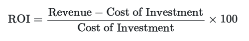
and the formula for ROAS is:
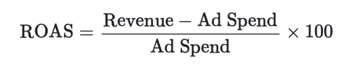
So you can see, they are very similar. We are just replacing Cost of Investment with Ad Spend, which is essentially the same thing. In these formulas we are calculating a fraction – the fraction earned from ad spend. For example, if you spent $20 on ads and they drove $100 in revenue, the ROAS would be $100-$20 = $80. Then we take the $80 and divide by $20 to get 4.
If we stopped there, we could say that you generate $4 in revenue for every $1 spent on advertising or a ROAS of 4:1. Industry benchmarks vary, but a ROAS above 3:1 is usually good (in the dataset I use below, it’s not that rosy – I should have used different numbers 🤷🏻). If we continue, we just multipy by 100 and get 400, or a 400% return on ad spend.
So, that is how you calculate ROAS. Now, using Python, we’re going to pull data from a database, caluclate ROAS, analyze & graph it, then add a little statistical seasoning to get some confidence intervals that give us a better read on the aggregated numbers (we tend to lose some stuff when we aggregate, so some additional numbers help us better understand the data, which gives us better information).
Getting the Data
First, we need some packages/modules/classes to help accompish this. I have commented next to the code so you can understand what each package/module/class does. What’s cool about Python is that you don’t have to import a whole package or module. For example, for datetime, we just need the datetime and timedelta classes (datetime is a module), so we can use from [package/module] import [module/class]. You can tell the difference between a package and module by running the following – print(pandas.__file__).
import pandas as pd # For data tables.
import numpy as np # For data arrays and typed data.
import matplotlib.pyplot as plt # To plot data.
import seaborn as sns # For stats visualisation.
from datetime import datetime, timedelta # For datetime data.
import psycopg2 #  PostgreSQL database adapter for Python.
Code language: PHP (php)
Next, we’re going to load some data. I’m going to use the data I created in Pt. 1 of this series (https://fujoconsulting.com/blog/data-driven-marketing-a-series-to-understanding-marketing-performance-pt-1-cpa/). That data is stored in a local PostgreSQL database. We’re going to open a connection to the database. Then pass a few SQL queries that will retrieve the data for us. We’ll assign them to pandas dataframes. Finally, we’ll close the connection.
# Create connection to db using psycopg2.
# SQLAlchemy is another, preferred way to connect, FYI.
conn = psycopg2.connect(
    host="localhost",
    database="postgres",
    user="postgres",
    password="Data123",
    port="5432"
)
Code language: PHP (php)
# Open cursor and test connection.
cursor = conn.cursor()
cursor.execute("SET search_path TO 'marketing_guide'")
# Get the data from the tables and assign a dataframe variable to each.
customers = pd.read_sql_query("SELECT * FROM marketing_guide.customers", conn)
marketing_spend = pd.read_sql_query("SELECT * FROM marketing_guide.marketing_spend", conn)
orders = pd.read_sql_query("SELECT * FROM marketing_guide.orders", conn)
attribution_touchpoints = pd.read_sql_query("SELECT * FROM marketing_guide.attribution_touchpoints", conn)Code language: PHP (php)# Close cursor & connection.
cursor.close()
conn.close()Code language: CSS (css)Calculating ROAS (feat. Python)
Now we have imported the data we’re going to use. We’ve assigned them to four pandas dataframes (customers, marketing_spend, orders, attribution_touchpoints).
Next, we’re going to create a function to calculate ROAS. We’re going to do this by channel. Then call the function and print the resulting dataframe data.
# Calculate ROAS by channel in a function - so it can be called repeatedly.
def calculate_roas(spend_data, customer_data, orders_data):

    # Get revenue by acquisition channel.
    # First join the customers to their orders.
    customer_orders = customer_data.merge(orders_data, on='customer_id')
    # Next, group the customers and their orders by acquistion channel.
    revenue_by_channel = customer_orders.groupby('acquisition_channel')['order_value'].sum().reset_index()
    # Finally, select only the channel and the revenue.
    revenue_by_channel.columns = ['channel', 'total_revenue']

    # Get spend by channel.
    # We have spend data, just need to aggregate it.
    spend_by_channel = spend_data.groupby('channel')['spend'].sum().reset_index()
    # and select only the channel and total_spend columns.
    spend_by_channel.columns = ['channel', 'total_spend']

    # Calculate ROAS.
    # First, join spend_by_channel to revenue_by_channel
    roas_data = spend_by_channel.merge(revenue_by_channel, on='channel', how='left')
    # Next, update NAs to 0
    roas_data['total_revenue'] = roas_data['total_revenue'].fillna(0)
    # Now, calculate ROAS (we're leaving out the * 100 part)
    roas_data['roas'] = roas_data['total_revenue'] / roas_data['total_spend']
    # Calculate profit
    roas_data['profit'] = roas_data['total_revenue'] - roas_data['total_spend']
    # Finally, calculate the profit margin.
    roas_data['profit_margin'] = roas_data['profit'] / roas_data['total_revenue']

    # Done! Return the roas_data dataframe.
    return roas_data

# Now we can call the function by passing in three of the dataframes
# we created by querying the database.
roas_analysis = calculate_roas(marketing_spend, customers, orders)

# and print the dataframe data.
print("ROAS Analysis:")
print(roas_analysis)
Code language: PHP (php)
ROAS Analysis:
channel total_spend total_revenue roas profit \
0 email_marketing 100.0 105.0 1.050000 5.0
1 facebook_ads 700.0 480.0 0.685714 -220.0
2 google_ads 1100.0 470.0 0.427273 -630.0
3 organic_search 0.0 730.0 inf 730.0
profit_margin
0 0.047619
1 -0.458333
2 -1.340426
3 1.000000
Code language: CSS (css)To get a clearer picture, we can create a graph and plot a bar chart, showing ROAS on the Y-axis and channel on the X-axis. I have to say, this is where I really miss R’s pipe operator – you can see we’re using “plt.” quite a lot. R has a solution, which is the |> (or + in ggplot) to join each line to next. Anywho, below is how we get our plot in pyplot.
# Visualize ROAS

# Set the size of the graph.
plt.figure(figsize=(12, 8))

# Arrange the channels from lowest ROAS to highest ROAS.
x_pos = np.arange(len(roas_analysis))[::-1]

# Select bar chart with the channel (x_pos) on the x-axis
# and the ROAS roas_analysis['roas'] on the y-axis
# add some colors and some labels.
plt.bar(x_pos,
        roas_analysis['roas'],
        alpha=0.7,
        color='skyblue'
)

plt.xlabel('Marketing Channel')
plt.ylabel('ROAS')
plt.title('Return on Ad Spend (ROAS) by Channel')
plt.xticks(x_pos, roas_analysis['channel'], rotation=45)
plt.show()
Code language: PHP (php)
That is basically it! However, we want to add a little more – we want to get a little better understanding of the data and what it’s trying to tell us. One way we can do that is by calculating the CIs (Confidence Intervals). These will give us an idea of how variable the data is below the aggregation. To do that, we create another function to calculate the CIs for the data.
# Function to calculate CIs.
def roas_significance_test(spend_data, customer_data, orders_data):
    results = [] # Empty list
    # Join customers to their orders by customer id.
    customer_orders = customer_data.merge(orders_data, on='customer_id')

    # Loop though each channel.
    for channel in spend_data['channel'].unique():
        # Sum the spend by channel.
        channel_spend = spend_data[spend_data['channel'] == channel]['spend'].sum()
        # Sum the revenue by channel.
        channel_revenue = customer_orders[
            customer_orders['acquisition_channel'] == channel
        ]['order_value'].values

        if len(channel_revenue) > 1:  # With only 1 revenue observation,
                                       # resampling with replacement would
                                       # give you the same single value every time.
            total_revenue = channel_revenue.sum() # Calculate revenue.
            roas = total_revenue / channel_spend # Calculate ROAS.

            n_bootstrap = 1000 # Number samples.
            bootstrap_roas = [] # new empty list.
            for _ in range(n_bootstrap): # Loop 1000 times.
                # By doing this 1000 times you build a distribution
                # of plausible ROAS values, which is what the CI is derived from.
                sample_revenues = np.random.choice(channel_revenue,
                                                   size=len(channel_revenue),
                                                   replace=True)
                # This creates a list that is the bootstrap distribution —
                # the raw material that np.percentile() then uses below
                # to calculate the CI bounds.
                bootstrap_roas.append(sample_revenues.sum() / channel_spend)

            # Then append the results and move to the next channel.
            results.append({
                'channel': channel,
                'roas': roas,
                'roas_95_ci_lower': np.percentile(bootstrap_roas, 2.5),
                'roas_95_ci_upper': np.percentile(bootstrap_roas, 97.5)
            })

    return pd.DataFrame(results)

# Call the function above.
roas_significance = roas_significance_test(marketing_spend, customers, orders)

# Print the results.
print("\nROAS Significance Testing:")
print(roas_significance)
Code language: PHP (php)
ROAS Significance Testing:
channel roas roas_95_ci_lower roas_95_ci_upper
0 google_ads 0.427273 0.327273 0.545455
1 facebook_ads 0.685714 0.228571 1.142857
2 organic_search inf NaN NaN
3 email_marketing 1.050000 0.900000 1.200000
Code language: CSS (css)Now that we have the CI data, we can add that to our graph. What I like is the CI (or error) bars with no middle marker (people tend to fixate on that). So, we’re going to join our ROAS data from the first graph with the CI data, then create a new graph and include the CI as an “errorbar”, a pyplot method, on each bar.
# Merge CI data into roas_analysis, preserving its channel order.
roas_plot = roas_analysis.merge(
    roas_significance[['channel', 'roas_95_ci_lower', 'roas_95_ci_upper']],
    on='channel',
    how='left'
)

# Build asymmetric error arrays: shape (2, N) — [lower_delta, upper_delta].
ci_lower_err = (roas_plot['roas'] - roas_plot['roas_95_ci_lower']).values
ci_upper_err = (roas_plot['roas_95_ci_upper'] - roas_plot['roas']).values
yerr = np.array([ci_lower_err, ci_upper_err])

# Plot, plot, plot...
plt.figure(figsize=(12, 8))
x_pos = np.arange(len(roas_plot))[::-1]

plt.bar(
    x_pos,
    roas_plot['roas'],
    alpha=0.7,
    color='skyblue',
    label='ROAS'
)
# Here's the addition of the errorbar.
# You can also adjust a number of things.
plt.errorbar(
    x_pos,
    roas_plot['roas'],
    yerr=yerr,
    fmt='none',  # No marker — error bars only.
    color='black',
    capsize=5,
    capthick=1.5,
    linewidth=1.5,
    label='95% CI (bootstrap)'
)

# And here's our plot with CIs.
plt.xlabel('Marketing Channel')
plt.ylabel('ROAS')
plt.title('Return on Ad Spend (ROAS) by Channel with 95% Confidence Intervals')
plt.xticks(x_pos, roas_plot['channel'], rotation=45)
plt.show()
Code language: PHP (php)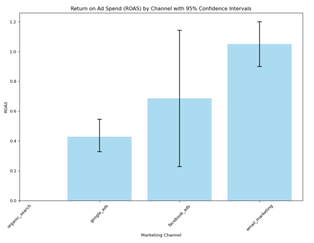
Conclusion
ROAS is simple to calculate, but it comes with a few caveats – measurement accuracy, proper tagging & tracking, and correctly aggregating data. You might already have a tool that does all this for you. However, it’s always a good idea to be able to calculate these KPIs on your own so you can ensure numbers are reported accurately.
Next in this series is something called LTV (Lifetime Value or Customer Lifetime Value – CLTV). Stay tuned!
About Us
We are Digital & Performance Marketing professionals. We help clients align marketing data, strategy & growth so that every decision, channel, and investment work together. If your data is disconnected, your strategy seems to be drifting, and your growth has been stalling, contact us today – we can help!