Data-Driven Marketing: A Series to Understanding Marketing Performance (Pt. 4

This article is also available on Medium.

Cohort analysis is the 4th in a series of 11 articles on performance marketing concepts and how to calculate them. This is not an exhaustive list of performance marketing concepts, but some of the key ones that can help you understand your marketing efforts and how they are performing. The list of concepts are listed below.

CPA (Cost Per Acquisition) – Channel efficiency analysis – one of the most important performance marketing metrics, representing the total cost to acquire one customer or conversion action.
ROAS (Return on Ad Spend) – Campaign profitability measurement – a revenue efficiency metric that measures how much revenue is generated for every dollar spent on advertising.
LTV (Customer Lifetime Value) – Predictive customer valuation – measures the total net profit a customer generates over their entire relationship with your business. It’s the foundation for determining how much you can afford to spend acquiring customers.
Cohort Analysis – Customer behavior tracking over time – a method of grouping customers by shared characteristics (typically acquisition date) and tracking their behavior over time to understand patterns in retention, revenue, and lifetime value.
Contribution Margin – True profitability assessment – the profit remaining after subtracting variable costs from revenue. It represents the amount available to cover fixed costs and generate profit, and critically for performance marketing, it determines how much you can afford to spend on customer acquisition.
Customer Segmentation – RFM and behavioral clustering – the practice of dividing your customer base into distinct groups that share similar characteristics, behaviors, or value profiles—enabling targeted strategies that improve acquisition efficiency, retention, and lifetime value.
Churn Prediction – Machine learning models for retention – uses historical customer behavior data to identify which customers are most likely to stop doing business with you, enabling proactive retention interventions before they leave.
Personalized Offer Scoring – Targeted campaign optimization – predicts which specific offer (discount level, product, message, timing, channel) to present to each individual customer to maximize business outcomes while minimizing unnecessary cost—essentially applying incrementality principles at the individual customer level.
Attribution Modeling – Multi-touch attribution including Markov chains – assigns credit for conversions across the multiple marketing touchpoints a customer encounters along their journey to purchase. It attempts to answer: “Which marketing activities actually drove this conversion?”
Cohort-Based LTV – Advanced lifetime value forecasting – measures the actual lifetime value of customers grouped by a shared characteristic (typically acquisition date or channel), tracking their real revenue and behavior over time rather than relying on aggregate or modeled estimates.
Order Economics – Transaction-level profitability analysis – the complete financial breakdown of an individual transaction—all revenue, costs, and resulting profit from a single order.

Understanding Cohort Analysis

Cohort analysis groups customers by shared characteristics and tracks their behavior over time. This reveals patterns in customer retention and value generation. These customers can be related by acquisition channel or campaign, or simply by date of first purchase. By grouping similar customers together, you can answers questions like:

How do retention rates vary by acquisition channel?
Which customer segments have the highest long-term value?
How does seasonality affect customer behavior?

My Experience With Cohorts

I remember first hearing about cohorts many years ago. A speaker was taking about them and I had a hard time understanding what they were. I related them to segments, which I understood. I thought “Are they just another word for segments? That can’t be right, can it?”. It took some time, but I began to see their value and how to define them.

Unlike segments, cohorts have a time value and a permanent association with the cohort. A customer in a high-value customer segment can move out of the segment, a customer can also move from one age group segment to another age group segment. A customer that made their first purchase in January of this year will not change. That cohort – customers that made their first purchase in January of this year – will remain the same group of customers. However, we can make things more interesting by adding a segment to the cohort, like high-value customers that made their first purchase in January of this year.

What makes cohorts interesting is their behavior over time. We can calculate their LTV (lifetime value), how many purchases they make, what types of purchases, return rates, etc. These calculations can be valuable in understanding our relationship to these cohorts and how we can best serve them.

Calculating Cohorts

To give an example of calculating cohorts, we’re going to use python and the data that I created in the first of this series, along with the additional data I added in the third article. Keep in mind that this is sample data – the real world will be noisier and sometimes make more, or less, sense. This data is stored locally in a PostgreSQL database, so we will need to retrieve the data so we can work with it.

Getting Started – Creating Tables

First, we will load the packages we need for this example:

import pandas as pd                               # tabular data manipulation
import matplotlib.pyplot as plt                   # low-level plotting primitives
import seaborn as sns                             # statistical visualisations built on matplotlib
from sqlalchemy import create_engine, text        # database connection pooling and raw SQL wrapper
import math       Code language: PHP (php)

Then we will connect to the PostgreSQL database, test the connection, retrieve the data, and then assign the SQL query results to pandas dataframes (don’t forget to disconnect from the database as well – in this case by using engine.dispose()):

# Create engine
engine = create_engine(
    "postgresql+psycopg2://postgres:Data123@localhost:5432/postgres",  # connects to local Postgres using psycopg2 driver
    connect_args={"options": "-csearch_path=marketing_guide"} # sets the default schema so table names need no prefix
)

# Test connection
with engine.connect() as conn:
    conn.execute(text("SELECT 1"))  # sends a trivial query to confirm the database is reachable

# Load data
with engine.connect() as conn:
    customers = pd.read_sql_query("SELECT * FROM customers", conn) # loads every row of the customers table into a DataFrame
    marketing_spend = pd.read_sql_query("SELECT * FROM marketing_spend", conn) # loads the marketing spend table
    orders = pd.read_sql_query("SELECT * FROM orders", conn) # loads the orders table
    attribution_touchpoints = pd.read_sql_query("SELECT * FROM attribution_touchpoints", conn)  # loads attribution touchpoints

engine.dispose()  # closes all connections in the pool now that loading is finishedCode language: PHP (php)

Cohort Analysis Function

Now we have a dataframe for each of the tables created in the PostgreSQL database: customers, marketing_spend, orders, and attribution_touchpoints. Next, we are going to create a function that we will pass in the customers & orders dataframes. The purpose of this function will be to combine the data, create the necessary cohort columns, and shape the data so we will be able to view and graph the cohorts. In this case, we will start with cohorts based on month of the year.

def comprehensive_cohort_analysis(customers_df, orders_df):
    # Merge customer and order data
    cohort_data = customers_df.merge(orders_df, on='customer_id') # joins every order to its customer record on customer_id
    cohort_data['first_purchase_date'] = pd.to_datetime(cohort_data['first_purchase_date']) # parses the first_purchase_date column as datetime so period extraction works
    cohort_data['order_date'] = pd.to_datetime(cohort_data['order_date']) # parses order_date as datetimeCode language: PHP (php)

We declare the function comprehensive_cohort_analysis, and pass two variables, which are the customers & orders dataframes, as customers_df, orders_df (so we don’t get confused :-)). The first thing we do in the function is join the customers and orders by customer_id. Then we need to convert the first_purchase_date & order_date to dates. These are often imported as character data and can be very difficult or impossible to work with if we don’t convert them to the proper datatype.

Next, we are going to create the cohort – year-month – for each order date and first purchase date:

    cohort_data['cohort_month'] = cohort_data['first_purchase_date'].dt.to_period('M') # truncates first purchase date to year-month, defining which cohort the customer belongs to
    cohort_data['order_month'] = cohort_data['order_date'].dt.to_period('M') # truncates each order date to year-month for period comparisonCode language: PHP (php)

Now that we have each order date and the first purchase date for each customer as year-month, we’re going to calculate each purchase period as an offset from the first purchase period. For example, a customer’s first purchase was in January and the second was in March, there is 1 purchase for period 0 and 1 purchase for period 2.

    cohort_data['period_number'] = (
    cohort_data['order_month'].apply(lambda x: x.ordinal) -    # converts each order's month to an integer offset from a fixed epoch
    cohort_data['cohort_month'].apply(lambda x: x.ordinal)  # subtracts the cohort's epoch offset, leaving the number of months elapsed since first purchase
    )Code language: PHP (php)

This creates a new column – period_number. Every customer has a first purchase and we can calculate how many customers had a first purchase in each period (year-month). What we’ll do now is create another dataframe with the period and the number of customers in each period. We’ll use this data to make some calculations in the next step:

    cohort_sizes = cohort_data.groupby('cohort_month')['customer_id'].nunique().reset_index() # counts distinct customers who first purchased in each cohort month
    cohort_sizes.columns = ['cohort_month', 'cohort_size'] # renames columns for clarityCode language: PHP (php)

Now that we have the cohort sizes by period and, separately, the cohort first purchase period, the current period, and customer id, we can group the customers by the cohort first purchase period and the current period, then join that to the dataframe we just created to calculate retention rates:

    retention_data = cohort_data.groupby(['cohort_month', 'period_number'])['customer_id'].nunique().reset_index() # counts how many distinct customers from each cohort placed an order in each period
    retention_data.columns = ['cohort_month', 'period_number', 'customers'] # renames columns

    # Merge with cohort sizes to calculate retention rates
    retention_data = retention_data.merge(cohort_sizes, on='cohort_month') # attaches the original cohort size to every row so we can compute a rate
    retention_data['retention_rate'] = retention_data['customers'] / retention_data['cohort_size']  # divides active customers in each period by the cohort's starting size to get a retention fractionCode language: PHP (php)

Next, we’ll add in revenue analysis and close the function with a return statement. This will return three dataframes: retention_data, revenue_data, and cohort_size to the caller:

    # Revenue analysis
    revenue_data = cohort_data.groupby(['cohort_month', 'period_number']).agg({
        'order_value': 'sum', # totals order value for each cohort-period bucket
        'customer_id': 'nunique' # counts distinct active customers in that bucket
    }).reset_index()
    revenue_data.columns = ['cohort_month', 'period_number', 'total_revenue', 'customers']  # renames aggregated columns
    revenue_data = revenue_data.merge(cohort_sizes, on='cohort_month') # attaches cohort size so revenue can be normalised per original member
    revenue_data['revenue_per_customer'] = revenue_data['total_revenue'] / revenue_data['cohort_size']  # divides total period revenue by full cohort size to get average revenue per original cohort member

    return retention_data, revenue_data, cohort_sizes  # returns all three computed DataFrames to the callerCode language: PHP (php)

That is the bulk of the code to process our cohorts. What we do now is call the function, which will return the dataframes for us to work with:

retention_analysis, revenue_analysis, cohort_sizes = comprehensive_cohort_analysis(customers, orders)

Retention Matrix

retention_analysis is the retention_data dataframe and we’re going to create a retention matrix to view the data:

retention_matrix = retention_analysis.pivot_table(
    index='cohort_month',    # each row is one acquisition cohort
    columns='period_number', # each column is one period offset (0 = acquisition month, 1 = one month later, etc.)
    values='retention_rate'  # cell value is the fraction of the cohort still purchasing in that period
)

print("Retention Rate Matrix:")  # labels the output block
print(retention_matrix)  # prints the cohort × period retention tableCode language: PHP (php)

That will give us a table of each period and the percent of customers that purchased again. For example, in the first row (2023-01), the first month was 1.0 or 100% – that is the first purchase and everyone has a first purchase – and the next month shows that 0.125 or 12.5% purchased again.

We can also graph this as a heat map, which I think is easier to view:

plt.figure(figsize=(15, 8))  # creates a new figure 15 inches wide and 8 inches tall
sns.heatmap(retention_matrix, annot=True, fmt='.2%', cmap='YlOrRd', mask=retention_matrix.isna())  # renders the matrix as a colour-coded heatmap; annotates each cell with its percentage value and leaves NaN cells blank
plt.title('Cohort Retention Rates') # sets the chart title
plt.xlabel('Period Number (Months)') # labels the x-axis
plt.ylabel('Cohort Month') # labels the y-axis
plt.show()    Code language: PHP (php)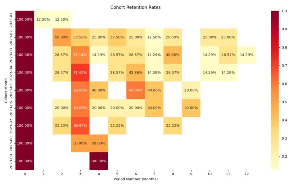

As you can see, this lines up with the retention rate matrix (but is easier to pick out stuff – like the 2023-09 cohort where they all bought again in the fourth period). With this matrix and graph, we can see repurchase rates; but what if we want to see the value of repurchase instead? Well, we have the revenue_analysis dataframe to help us with that.

Revenue Matrix

What we’ll do is the same as above, but with the revenue_analysis dataframe instead of the retention_analysis dataframe:

revenue_matrix = revenue_analysis.pivot_table(
    index='cohort_month',  # each row is one acquisition cohort
    columns='period_number',  # each column is one month offset
    values='revenue_per_customer'# cell value is average revenue per original cohort member in that period
)

# Calculate cumulative LTV
cumulative_ltv_matrix = revenue_matrix.cumsum(axis=1) # running sum across columns so each cell shows total revenue earned from period 0 through that period

print("\nCumulative LTV Matrix:")  # labels the output block
print(cumulative_ltv_matrix) # prints the cohort × period cumulative LTV tableCode language: PHP (php)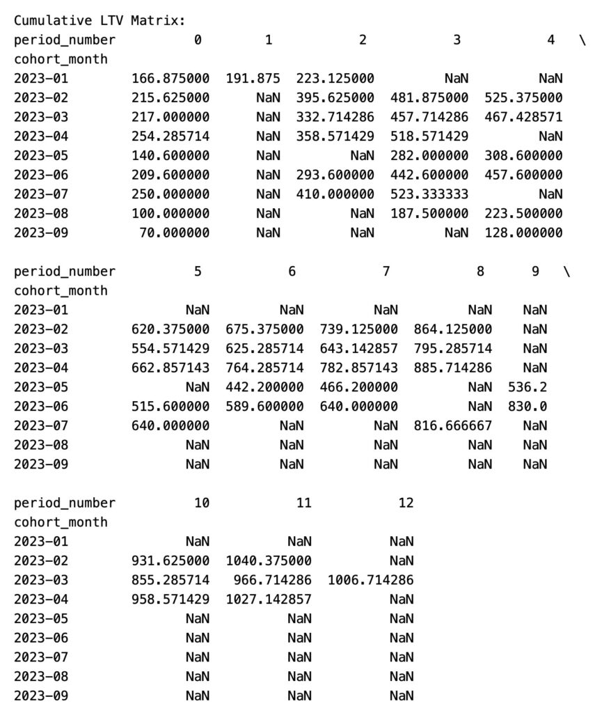

We could also do a heatmap for this this, however, it might be more informative to create a cumulative LTV chart. Let’s do that instead:

plt.figure(figsize=(12, 8)) # creates a new 12 × 8 inch figure
for cohort in cumulative_ltv_matrix.index: # iterates over each cohort row
    plt.plot(cumulative_ltv_matrix.columns, cumulative_ltv_matrix.loc[cohort],
            marker='o', label=f'Cohort {cohort}') # plots that cohort's cumulative LTV over time with circle markers

plt.title('Cumulative Customer Lifetime Value by Cohort')  # sets the chart title
plt.xlabel('Months Since First Purchase') # labels the x-axis
plt.ylabel('Cumulative LTV ($)') # labels the y-axis
plt.legend() # adds a legend identifying each cohort line
plt.grid(True, alpha=0.3) # adds faint grid lines for readability
plt.show()        Code language: PHP (php)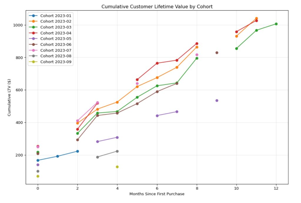

Very quickly we can see the trend and value of each cohort, with 2023-02, 2023-04, and 2023-03 the most valuable cohorts in the data over time.

Summary

I hope this gave you a good overview of what cohort analysis is and how you can do it yourself. As you can see, it can be a powerful way to understand your customers and customer trends. Additionally, you can add segmentation to further drill into cohorts for greater insights.

In my next article in this series, I’m going to dive into contribution margin. As we look at LTV, we also need to understand profit and costs and what true profitability looks like. Stay tuned!

At Fujo, we help you align data, strategy and growth. If you are having trouble with segmentation and understanding the impact of various cohorts, we can help wrangle your data.

If you’re not able to make sense of your marketing cohorts, data is hard to access or spreadsheets are overwhelming you – we can simplify your efforts with real impact.

We work with brands to identify where performance is being lost across the system and uncover opportunities that do not show up in standard reporting.

If you are interested, we are always open to a conversation.

Data-Driven Marketing: A Series to Understanding Marketing Performance (Pt. 4 — Cohort Analysis)